-
The building modal displacement demand (performance point) is calculated automatically as a result of the pushover analysis.
ICONS
a y1 = Yield pseudo-acceleration for the first mode [m/s 2 ]
C R = Spectral displacement ratio
d 1,max (X) = Maximum displacement (performance point) of the modal single degree-of-freedom system for the (X) earthquake direction [m]
f e = Calculated linear (elastic) strength demand for the structural system
f y = Projected ductility capacity and period dependent yield strength
S ae (T 1 ) =Linear elastic spectral acceleration corresponding to the first natural vibration period T 1 [g]
S de (T 1 ) = the first natural vibration period T 1 'to the corresponding linear elastic spectral displacement [m]
S di (T 1 ) = the first natural vibration period T 1 ' to the corresponding non-linear spectral displacement [m]
T B = Horizontal elastic design acceleration spectrum corner period [s]
T 1 = Natural vibration period of the first mode [s]
μ(R y ,T 1 ) = Yield Strength Reduction Coefficient and ductility demand calculated according to the first natural vibration period
ω1 (1) = First mode natural angular frequency[rad/s]found from the free vibration calculation, which is renewed at each kth thrust step
Earthquake modal displacement demand 's to obtain, under the effect of earthquake modal capacity represented by the diagram of modal single degree of freedom systems to maximum displacement of ' corresponds to the account. The earthquake effect is found using the Horizontal Elastic Design Spectrum, and the maximum displacement of the modal single degree of freedom system is found by using the modal capacity curve obtained as a result of the pushover analysis . The modal displacement demand of the earthquake , the performance point in the thrust curve also called. At this point of the thrust analysis, the plastic deformation values calculated in the elements are compared with the limit values, and the building performance is determined.
In a modal single degree of freedom system, the largest displacement is defined as a nonlinear spectral displacement as in TDY Equation 5.12 .

In this equation, d 1, max (X) , modal largest displacement of a single degree of freedom system , expand S di (T 1 ) the first natural vibration period of the carrier system T 1 'to the corresponding non-linear spectral displacement ' y refers to. The value of S di (T 1 ) is defined by TBDY Equation 5B.13 .

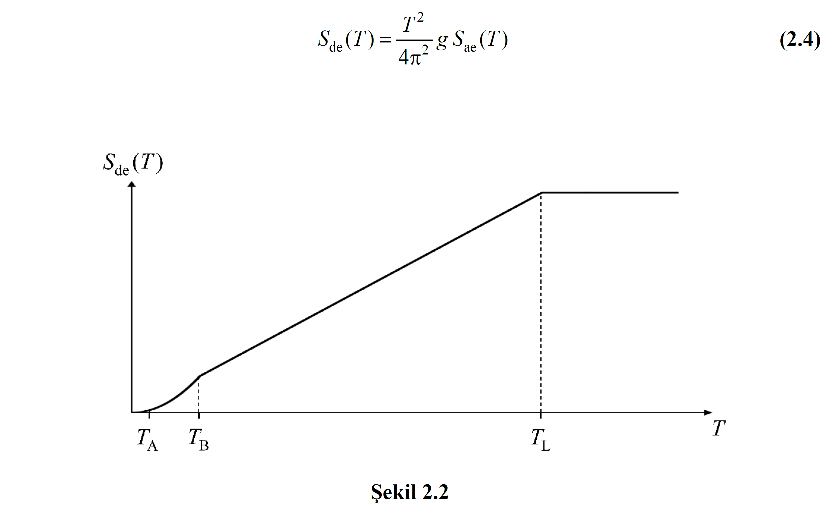
In this equation, S in (T 1 ) , TDY Equation 2.4 as defined by the natural vibration period corresponding to the first elastic displacement of spectral design 'is.
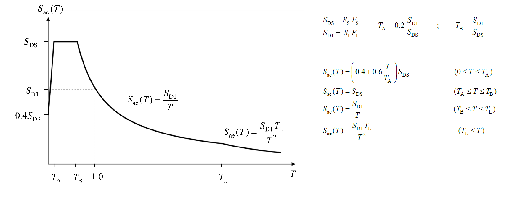
The S ae (T 1 ) value is the horizontal elastic design spectral acceleration, which is the ordinate of the Horizontal Elastic Design Spectrum .
Equation TDY 5B.13 'in the C R , spectral displacement ratio' n shows and TDY 5B.14 equation is defined by.

In this equation, R y , yield strength reduction factor 'n is shown. In the DGT approach, TDY is a size that is directly obtained as a result of the yield strength as a result of the thrust calculation in the TDGT approach, unlike a size defined in Annex 4A , depending on the ductility capacity, and TDY is expressed by Equation 5B.15 .

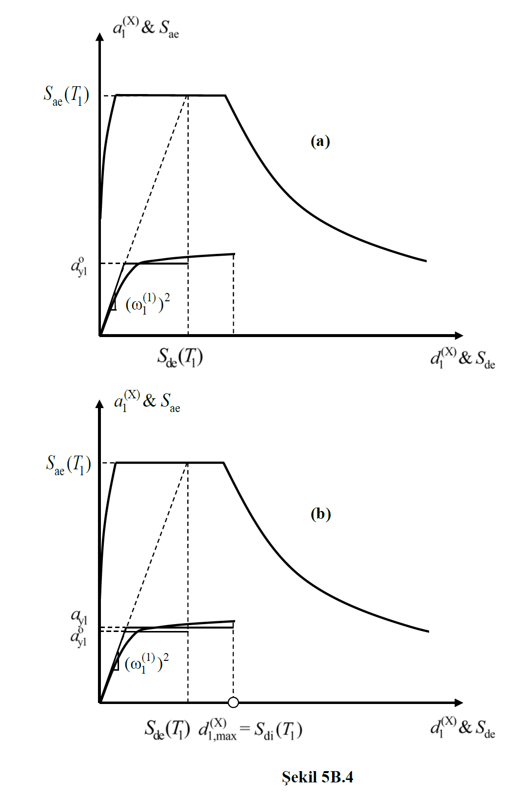
In this relation f e and S aa (T 1 ) elastic strength demand 's and her corresponding elastic response spectrum ' t, f y and a y1 The yield strength 's and opposed it flows so-called acceleration ' n represents ( TDY Figure 5B.4 ). In this equation, the S ae (T 1 ) value is the linear earthquake spectrum obtained by transforming the Horizontal Elastic Design Spectrum , whose coordinates are modal displacement - modal pseudo-acceleration . is the ordinate.
Equation TDY 5B.14 'in point μ (R y , T 1 ) , yield strength ' due to the natural vibration period, and that the expressed Ductility Demand 'is. For the calculation of this magnitude , the relations in Equation 5B.16 can be obtained by writing the relations in Equation 4A.2 given in TDY Annex 4A in reverse order .
(a) The ductility demand of the earthquake, μ(R y ,T 1 ), is taken as equal to the Yield Strength Reduction Coefficient R y for structural systems with less rigidity in accordance with the equal displacement rule .

(b) For structural systems with more rigidity , the equation in Equation 5B.16b is obtained from Equation 4A.2b :

5B.16 equation 'benefiting from the relationship in equation 5B.14 ' t defined by the spectral displacement ratio C R , TDY equation 5B.17 'is expressed as in FIG.

Equation 5B.12 indicated at the largest displacement of the modal single degree of freedom system d 1, max (X) , fixed Single Mode Jacking Method or Variable Single Mode Jacking Method coordinates obtained using the spectral displacement - modal so-called acceleration which modal capacity diagram building on It is the horizontal component of the performance point that determines its performance. 5B.12 equation according to the horizontal elastic design spectrum 's which is led by converting coordinates and spectral displacement - spectral acceleration (S in , S aa ) which The S di (T 1 ) value on the horizontal axis of the linear earthquake spectrum and the modal displacement value d 1,max (X) of the performance point are equal. The superimposition of these two graphs is shown in TDY Figure 5B.3 .
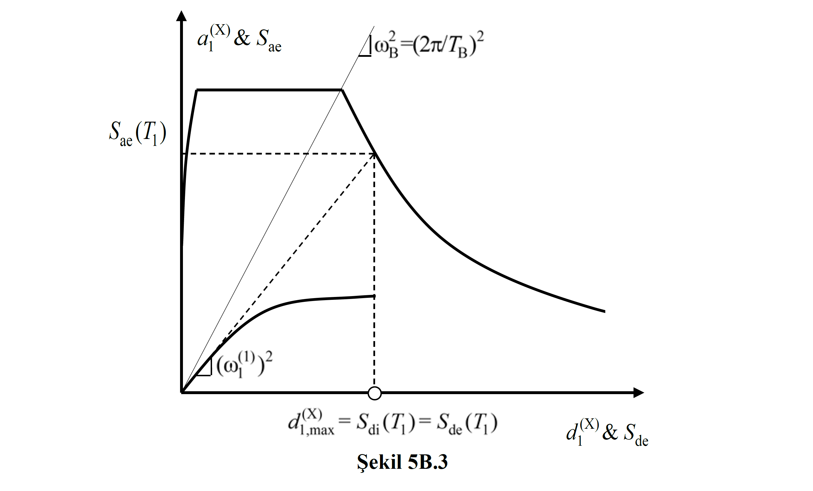
Figure 5B.3 TDY 'in the condition illustrated in Equation 5B.13 with Equation 5B.17 ' corresponds to the implementation. In this case, it is sufficient to show that the natural vibration period in the first impulse step, without any operation on the modal capacity curve, meets the condition T 1 >T B or (ω 1 (1) ) 2 ≤ ω B 2 . Wherein the initial slope (ω 1 (1) ) the second value of the natural vibration period of the building dominant T 1 's T B ' means that greater than. In this case TDY Equation 5B.17aapplying spectral displacement ratio C R = 1 is received, and d 1, max (X) = S in (T 1 ) is calculated.
On the other hand, the natural vibration period of the building dominant T 1 's T B from A is smaller ( Figure 5B.4 ' in the illustrated case), Equation 5B.13 with Equation 5b.17b 'corresponds to the implementation. In this case the spectral displacement ratio C R calculated in the sequential approach. For this purpose modal capacity diagram , figure 5b.4 A as depicted in prior C R = 1 two rectilinear taking elastoplastic converted to a diagram. The equality of the areas under the diagrams is taken as basis in the transformation process. Approximate yield pseudo-acceleration found in this way a y1 ousing Equation 5B.15 from the R y and hence Equation 5b.17b from the C R and Equation 5B.13 'skin S di (T 1 ) is calculated. Accordingly, the elasto-plastic diagram is reconstructed ( Figure 5B.4b ) and the same operations are repeated based on the re-found a y1 . At the step where the results are close enough, the sequential approach is terminated.