
ICONS
a y1 = Yield pseudo-acceleration for the first mode [m/s 2 ]
C R = Spectral displacement ratio
d 1,max (X) = Maximum displacement of the modal single degree-of-freedom system for the (X) earthquake direction [m]
f e = Carrier Calculated linear (elastic) strength demand for the system
f y = Projected ductility capacity and period-dependent yield strength
S ae (T 1 ) =Linear elastic spectral acceleration corresponding to thefirst natural vibration period T 1 [g]
Sde (T 1 ) =Linear elastic spectral displacement [m] corresponding to thefirst natural vibration period T1
S di (T 1 ) =Nonlinear spectral displacement corresponding to thefirst natural vibration period T1[m]
T B = Horizontal elastic design acceleration spectrum corner period [s]
T 1 = Natural vibration period of the first mode [s]
μ(R y ,T 1 ) = Yield Strength Reduction Coefficientandductility demandcalculated according to the first natural vibration period
ω 1(1) = First modenatural angular frequency[rad/s]found from the free vibration calculation, which is renewed at each kth thrust step
5.6.5. Obtaining the Modal Displacement Demand of the Earthquake in Single-Mode Pushover Analysis Methods
5.6.5.1 - Earthquake modal displacement demand 's to obtain, under the effect of earthquake modal capacity diagram represented by modal single degree of freedom systems to maximum displacement of ' corresponds to the account.
5.6.5.2 – The modal displacement demand of the earthquake;
(a) Modal can be obtained as Nonlinear Spectral Displacement in a single degree of freedom system .
(b) It can be obtained from the time history calculation of a modal single degree-of-freedom system under earthquake effect. Both methods are described in Appendix 5B .
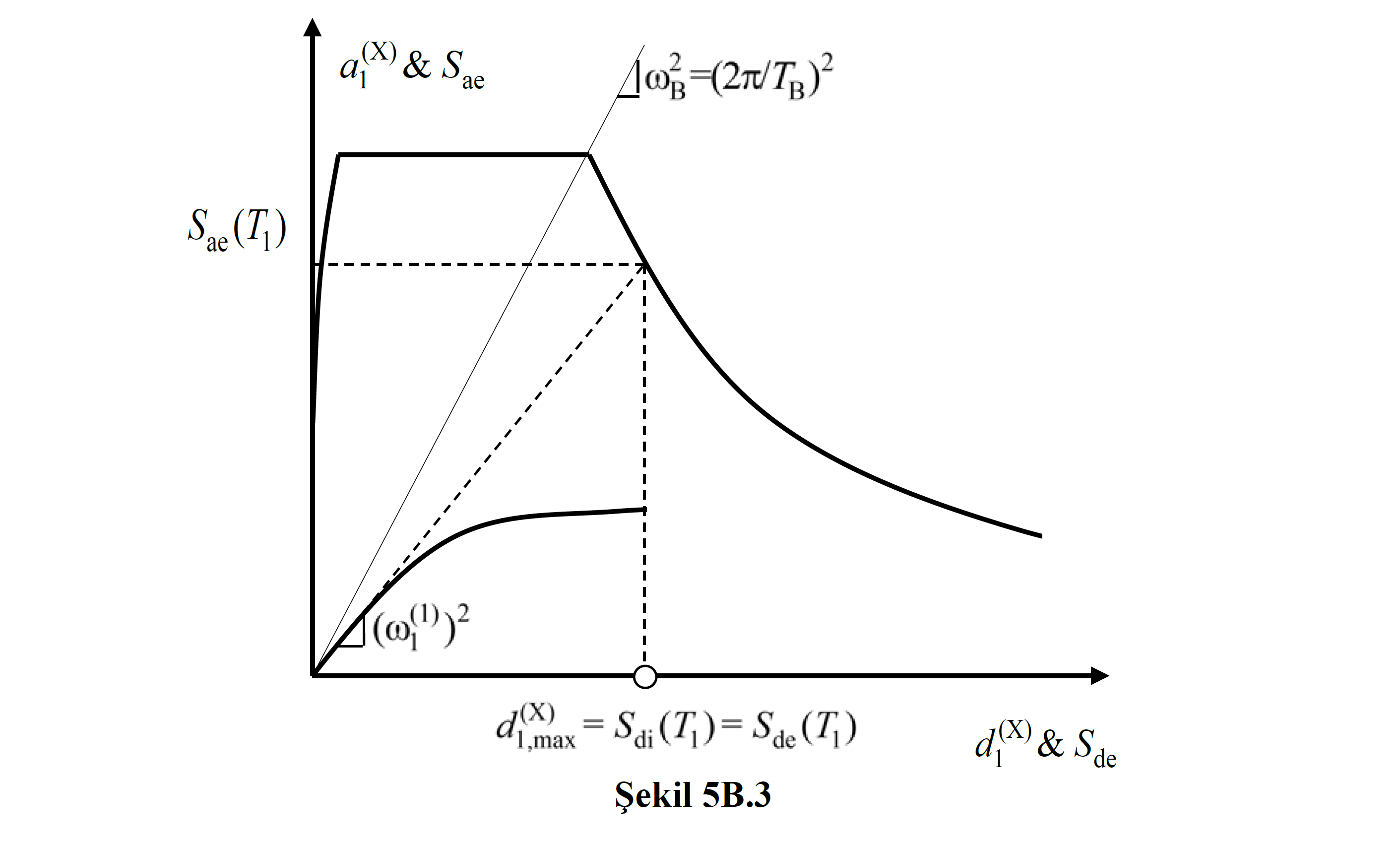
5B.3. ACQUISITION OF THE EARTHQUAKE'S MODAL REPLACEMENT DEMAND AS NONLINEAR SPECTRAL DISPLACEMENT
Earthquake modal displacement demand 's to obtain, under the effect of earthquake modal capacity diagram represented by a single degree of freedom systems to maximum displacement of modal ' corresponds to the account.
5B.3.1 – In a modal single degree of freedom system, the largest displacement is defined as a nonlinear spectral displacement:

Here, d 1, max (X) of the modal single degree of freedom systems to maximum displacement of 'n, S di (T 1 ) of the conveyor system of the first natural vibration period T 1 ' and corresponding to Eq. (5B.13) defined by non-linear spectral indicates displacement .

S wherein the (T 1 ), Eq. (2.5) defined by the elastic displacement of spectral design , expand C R In Eq. (5B.14) 't defined by the spectral displacement ratio ' n is Impr.
5B.3.2 - Eq. (5B.13) 'in point spectral displacement ratio C R , Eq. (5B.14) have been identified:

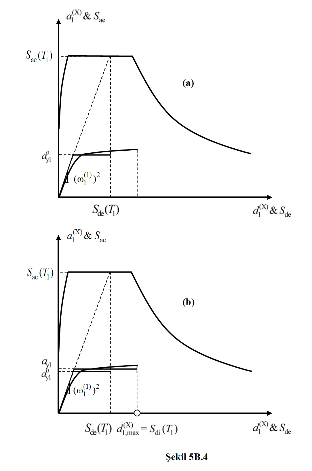
Wherein the yield strength reduction factor 'n indicating R y , Design by Solidarity to approach EK 4 ' unlike the definition given in predicted not a quantity which is defined depending on the ductility capacity, directly obtained from a thrust account the resistance to flow 's-dependent magnitude represents:

In this relation f e and S aa (T 1 ) elastic strength demand 's and her corresponding elastic response spectrum ' y, f y and y1 is the yield strength 's and her corresponding flow pseudo-acceleration ' n represents ( Figure 5B.4 ).
5B.3.3 – μ(R y ,T 1 ) in Eq.(5B.14) is the ductility demand expressed depending on the yield strength and the natural vibration period . To account for this size ANNEX 4 'in Eq. (4A.2) with the reverse relations are obtained by writing the relation:
(a) Seismic ductility demand μ (R y , T 1 ), equal displacement rule in accordance with the stiffness of not more for carrier systems Yield Strength Reduction Factor R y 'is taken equal to:

(b) For carrier systems with more rigidity, the equation in Eq.(5B.16b) is obtained from Eq.(4A.2b) :

5B.3.4 - Eq. (5B.14) 't defined by the spectral displacement ratio C R , Eq. (5B.16) from utilizing Eq. (5B.17) wherein is expressed as:

5B.3.5 – The modal capacitance diagram belonging to the first (dominant) vibration mode in Figure 5B.3 and Figure 5B.4 and whose coordinates are modal displacement–modal pseudo-acceleration (d 1 ,a 1 ) and its coordinates spectral displacement–spectral acceleration ( The linear earthquake spectrum with S de , S ae ) was drawn together.
(a) The situation shown in Figure 5B.3 corresponds to the application of Equation (5B.17a) together with Equation (5B.13) . In this case, without doing anything on the modal capacitance diagram, it is sufficient only to show that the natural vibration period in the first impulse step satisfies the condition T 1 >T B or ( (1) 1 (1) ) 2 ≤ 2 B 2 .
(b) On the other hand , the situation shown in Figure 5B.4 corresponds to the application of Equation (5B.17b) together with Equation(5B.13) . In this case the spectral displacement ratio C R will be calculated in the sequential approach. For this purpose modal capacity diagram, figure 5b.4 A as depicted in prior C R = 1 two rectilinear taking elastoplastic converted to a diagram. The equality of the areas under the diagrams is taken as basis in the transformation process. From Eq.(5B.15) using the approximate yield pseudo-acceleration a y1 o found in this way, R y and accordinglyEq. (5b.17b) from the C R and Eq. (5B.13) 'skin S di (T 1 ) is calculated. Accordingly, the elasto-plastic diagram is reconstructed (Figure 5B.4b) and the same operations are repeated based on the re-found a y1 . At the step where the results are close enough, the sequential approach is terminated.
5B.3.6 - Earthquake modal displacement demand 's in Eq. (5B.13) and Eq. (5B.17) ' benefiting from Eq. (5B.12) according to the calculation (a) and (b) as defined in cases are not applicable.
(a) In cases where the distance of the nearest fault to the building is less than 15 km, calculation will be made in the time history according to 5B.4 using near-field earthquake records selected and scaled according to 2.5 .
(b) In case the post-yield slopes of the modal capacity diagram are negative due to second order effects , the calculation will be made in the time history according to 5B.4 using earthquake records selected and scaled according to 2.5 .
Related Topics