
After the function definitions are made, an analysis situation should be created for each function in the X and Y directions. The analysis case definition basically includes time intervals, input functions definitions and Rayleigh damping ratio statement.
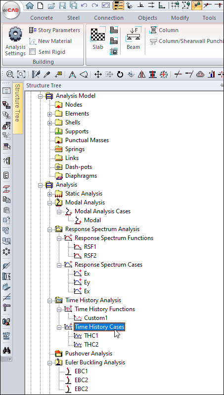
The time history states are displayed in the structure tree under the Analysis folder.
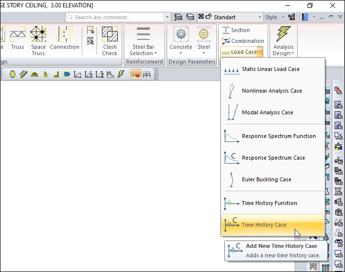
Location of Time History Case Command
You can access it from the ribbon menu, Analysis and Design tab, under the Define heading.
Usage Steps
-
First, define the time history function as described in the previous topic .
-
Click the time history case icon.
-
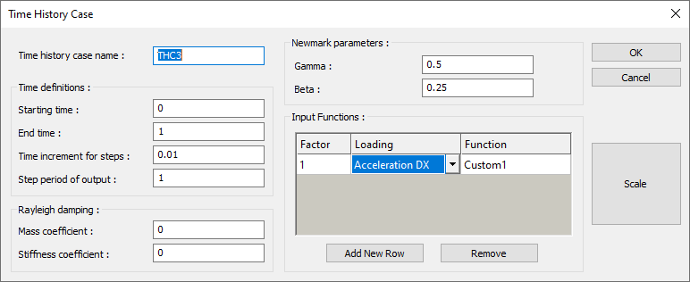
The Time History Case dialog will open.
-
Click the Add New Row button in the Input Functions section.
-
Custom 1 will appear in the Function column. For example, choose acceleration DX as the download.
-
Enter the scale factor of the acceleration register as the actor.
-
Enter the mass coefficient and stiffness coefficient values.
In dynamic analysis, the damping ratio is reflected in the calculation with the damping coefficient. In the time history analysis, it is taken into account with the Rayleigh damping equation. The equation consists of mass and stiffness coefficients, and these coefficients vary according to the structure.
Mass coefficient = a0= 2.ξi.ωi − a1.ωi ωi
Stiffness coefficient= a1= (2.ξj.ωj – 2.ξi.ωi)/( ωj ωj -ωi ωi )
I, j = First and last period values of the structure.
ξi, ξj = The damping ratios of the structure in the i and jth periods. 5% can be taken.
ωi, ωj= are the i and jth angular frequencies of the structure.
-
In my time definitions section, give the starting, end times, time increment for steps, step period of output.
-
Click the OK button to close the dialog.
|
Specifications |
|
Time history case name The case name is entered. |
|
Starting time The starting time is entered. |
|
End time The end time is entered. |
|
Time increment for steps The value for the time increment is entered at each step. |
|
Step period of output Step period is entered for outputs. |
|
Mass coefficient Mass coefficient is entered. |
|
Stiffness coefficient Stiffness coefficient is entered. |
|
Gamma Gamma value is entered. |
|
Beta Beta value is entered. |
|
Input functions 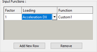
From the loading column, determine which loading or loadings you will do the analysis for and enter a factor. You can add uploads one after the other with add new row. |
|
Scale 
It is a scaling method used to approximate the acceleration record defined in the time history function to the elastic design spectrum curve. In this method, only a single acceleration record is scaled by zooming into the spectrum curve. For three-dimensional calculation, you can use the Scale Ground Motion command under Analysis list from the Ribbon menu. 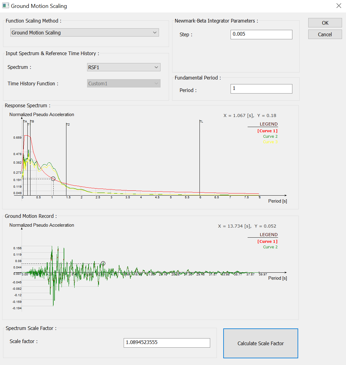
|
Next Topic