-
Scaling of the selected earthquake acceleration records is done automatically with the simple scaling method.
-
The number of earthquake record sets and selection of earthquake records for three-dimensional calculations are under user control
ICONS
T p = Dominant natural vibration period of the building
Appropriate earthquake records should be selected and scaled in order to define the earthquake ground motions required in three-dimensional earthquake calculation in the time domain of building carrier systems.
According to Section 2.5.1 of TBDY , the selection of earthquake records to be used in earthquake calculation in the time domain of the building carrier systems will be made by considering the earthquake magnitudes compatible with the earthquake ground motion level, fault distances, source mechanisms and local ground conditions. The number of earthquake record sets to be selected for three-dimensional calculation should be at least eleven. The number of recording and recording sets to be selected from the same earthquake shall not exceed three.
Calculation in time history is applied in two different ways in ideCAD Static.
-
The first is the Earthquake Calculation with Mode Addition Method in the Time History Area , which is described in TBDY Section 4.8.3 . Details of the method are explained in TBDY ANNEX 4B.3 . This method is one of the modal calculation methods used in the Design Based on Strength approach , DOT approach. With this calculation method, linear earthquake calculation is made.
-
The second method is Linear Analysis in the Time Domain .
According to TBDY Section 2.5 , if any three-dimensional earthquake calculations are made in the Time History Area, the earthquake records should be scaled or converted to provide spectral matching.
The simple scaling method is to change the amplitudes of the selected earthquake acceleration records by multiplying them by a constant coefficient to comply with the Horizontal Elastic Design Spectrum . In this method, since the amplitudes of the earthquake acceleration records are multiplied by a constant coefficient, there is no change in the frequency of the earthquake acceleration.
According to TBDY Section 2.5.2 , scaling of earthquake records for three-dimensional calculations with simple scaling method is done in the following order.
-
As a first step, the spectrum of each earthquake acceleration record is obtained.
-
The resultant horizontal spectrum is obtained by taking the square root of the sum of the squares of the spectra of the two horizontal components of each earthquake record set.
-
The Horizontal Elastic Design Spectrum described in TBDY Section 2.3.4 is selected as the target spectrum.
-
For each resultant horizontal spectrum, the scale coefficient where the difference between the target spectrum amplitudes is minimum is calculated.
-
The amplitude of each of the eleven resultant horizontal spectra is multiplied by the scale coefficient.
-
The ratio of the average of the resultant spectra of all the scaled records between the 0.2T p and 1.5T p periods to the amplitudes of the Horizontal Elastic Design Spectrum in the same period is checked whether it is less than 1.3.
-
When this ratio is greater than 1.3, scale coefficients are found for eleven sets of earthquake acceleration records.
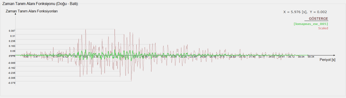
The picture below shows eleven sets of acceleration registers scaled with the simple scaling method.
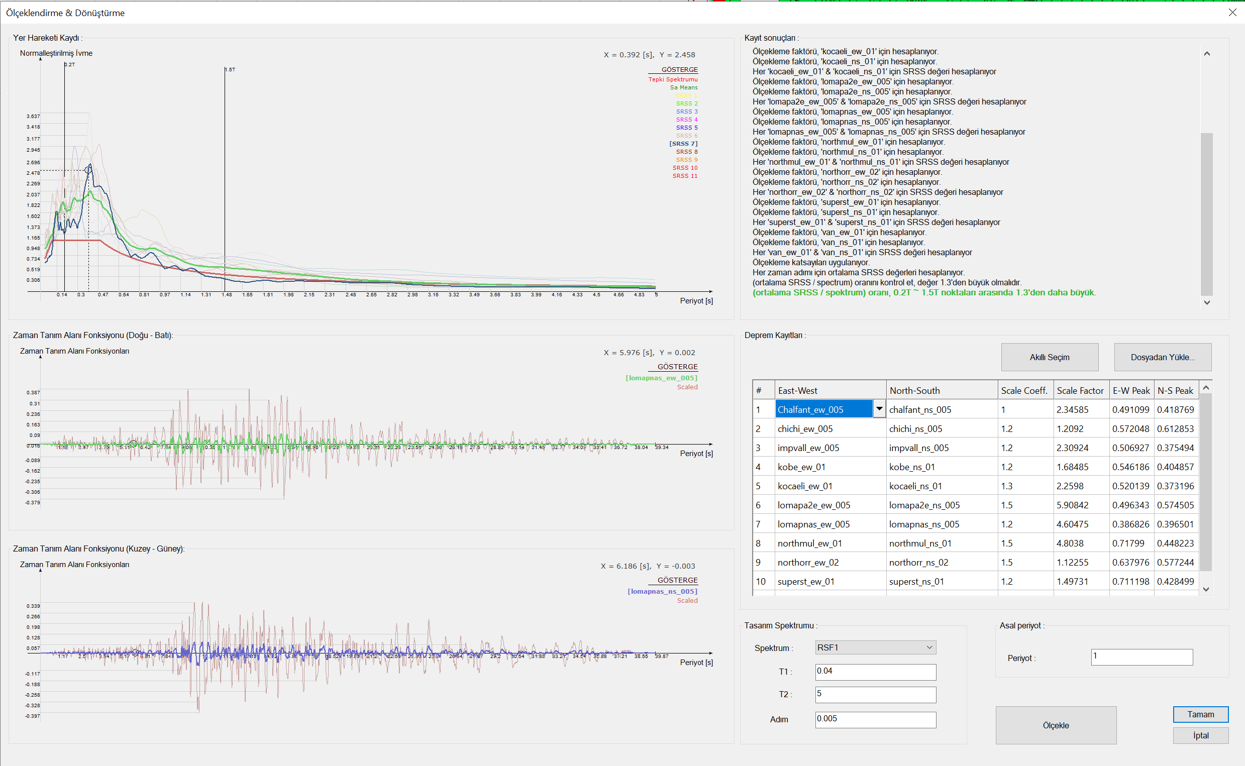
Scaled and unscaled acceleration registers are shown separately, as seen in the picture above. In the picture below, the unscaled version of the graphical acceleration record is shown in green, and the scaled version of the acceleration record is shown in red.
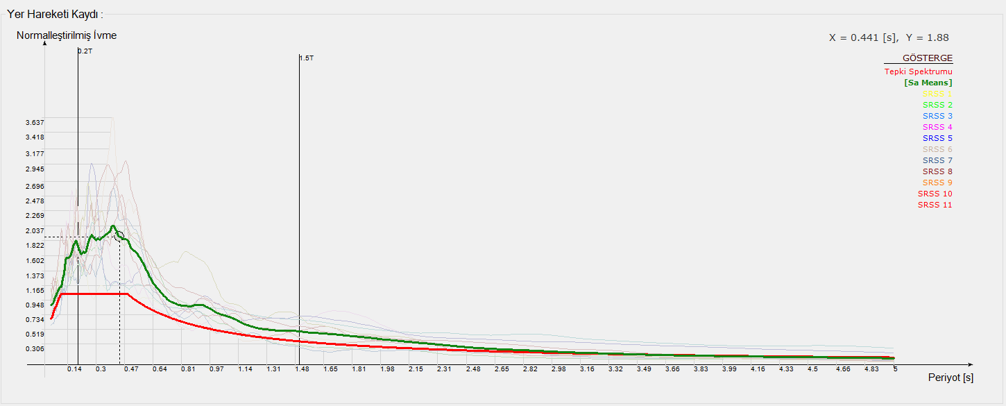
A comparison of the average spectra of eleven acceleration registers with the Horizontal Elastic Design Spectrum is shown in the picture below. The graph shown here in green is the mean of the scaled resultant horizontal spectra. The graph shown in red is the horizontal elastic design spectrum. These two graphs were compared between the 0.2T p and 1.5T p periods and it was seen that the ratio of the amplitudes was greater than 1.3.