
-
Live Load Mass Participation Coefficient, n which is used to determine the horizontal earthquake effect E d (H) of the evaluation of the structural system elements , is selected based on the user control according to Equation 4.9 according to 4.4.2.1 .
-
After the Live Load Mass Participation Coefficient, which is used in determining the horizontal earthquake effect , is selected by the user, the thrust analysis is performed automatically by the program.
-
Static vertical loads, nonlinear static calculations that take the second order effects incrementally applied to the carrier system into account are applied automatically. The internal forces and deformations obtained from this calculation are automatically taken into account in the initial condition of the repulsion analysis.
-
Nonlinear deformations are automatically taken into account as the initial condition in new buildings and in the evaluation of existing buildings.
ICONS
E d (H) = Horizontal earthquake effect based on the design with directional coupling
E d (X) = earthquake effect in the direction of (X)
E d (Y) = earthquake effect in the direction of (Y)
E d (Z) = Vertical earthquake effect
G = Constant load effect
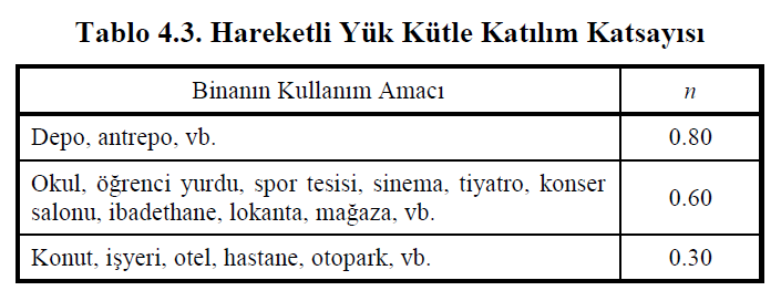
n = Live load participation coefficient
Q = Live load effect
Q e = Effectiveliveload effect
S = Snow load effect
As explained in Article 5.2.2.1 of TBDY, the combination of earthquake effect with vertical load effect is made with the following equation.

This equation shows G constant load effect, Q e effective live load effect, S snow load effect, E d (Z) vertical earthquake effect, E d (H) horizontal earthquake effect.
The effective live load effect Q e is calculated using the Live Load Mass Participation Coefficient, n, defined in Table 4.3 TBDY . It is calculated as Q e = nQ, where Q is the live load effect .
E d (H) represents the horizontal earthquake effect. If the Shaping Assessment and Design (ŞGDT) approach is applied to the structure, the horizontal earthquake effect should be defined as in Article 5.2.2.3 of TBDY . If any of the pushing methods given in Section 5.6 of TBDY are applied to the system , the earthquake effects in the E d (H) , (X) and (Y) directions are calculated separately and then combined according to TBDY Section 4.4.2.1 . The earthquake effects defined in horizontal (X) and (Y) directions perpendicular to each other according to Section 4.4.2.1 of TBDY are combined as described in Equation (4.9) .

In this case, 8 different impulse calculations emerge when the push analysis is made for any structure. For example, the pushover analysis combinations applied to a house (n = 0.3) without snow load should be as follows.
G + 0.3Q + E d (X) + 0.3E d (Y) + 0.3E d (Z) G + 0.3Q + E d (Y) + 0.3E d (X) + 0.3E d (Z)
G + 0.3Q + E d (X) -0.3E d (Y) + 0.3E d (Z) G + 0.3Q + E d (Y) -0.3E d (X) + 0.3E d (Z)
G + 0.3QE d (X) + 0.3E d (Y) + 0.3E d (Z) G + 0.3QE d (Y) + 0.3E d (X) + 0.3E d (Z)
G + 0.3QE d (X) -0.3E d (Y) + 0.3E d (Z) G + 0.3QE d (Y) -0.3E d (X) + 0.3E d (Z)
TBDY Article 5.2.2.2 according to the assessment and design according to Strain structure (ŞGDT) approach is implemented, will be non-linear calculation method of seismic analysis (any push analysis or time domain non-linear analysis) is preceded M d (H Nonlinear static calculation in which static vertical loads other than ) are applied incrementally to the carrier systemwill be made. Internal forces and deformations obtained from this calculation are taken into account as the initial value in the horizontal earthquake calculation. In this case, the nonlinear static calculation applied using the vertical loads is made according to the following loading condition. Internal forces and deformations obtained as a result of this analysis are considered as the initial value of the horizontal earthquake calculation.
G + nQ + 0.2S + 0.3E d (Z)
In this loading case, n is the Live Load Mass Participation Coefficient as described above and it is calculated from Table 4.3. For example, a non-linear static calculation applied incrementally under the following loading condition is performed as the initial step (i = 0) before the push analysis is applied to a house (n = 0.3) without snow load .
G + 0.3Q + 0.3E d (Z)
In this nonlinear static calculation , the nonlinear behavior of the structure in terms of geometry and material is taken into account.
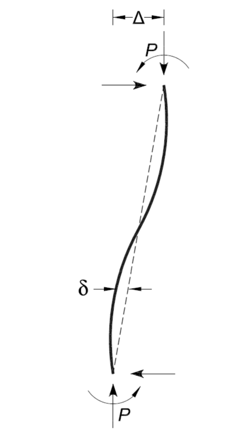
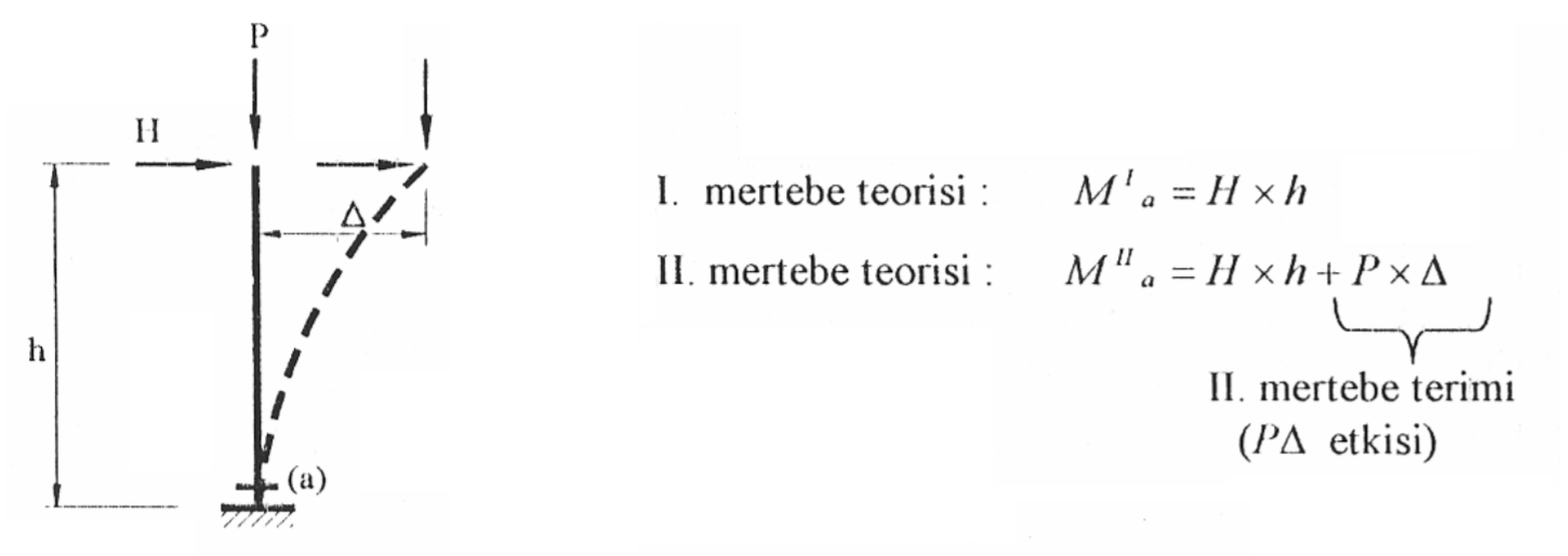
In the nonlinear analysis in terms of geometry, second-order effects arising due to axial forces occurring in structural elements are taken into consideration. Second order effects are divided into two as p-δ and p-Δ. The figure on the right is a representational representation of how p-δ and p-Δ effects occur in an element. The p-δ effect is caused by the axial pressure force on the element trying to increase the displacement caused by the curvature of the element itself. The p-Δ effect, on the other hand, creates additional moments in the element due to the axial pressure force due to the displacements of the joints of the element. p-Δ is explained in more detail in the image below.
Details of the nonlinear analysis in terms of material are explained in detail under the titles Concentrated Plasticity Model and Distributed Plasticity Models. According to Article 5.2.2.2 of TBDY , if there is a plasticization situation in the nonlinear analysis performed under the effect of vertical loads, G + nQ + 0.2S + 0.3E d (Z), this situation is not allowed in new buildings and reinforced buildings. However, nonlinear deformations (plastic joints) are taken into account as the initial value if the ŞGDT approach is applied to evaluate existing buildings.
Next Topic